Generation and publication of Machine Learning models

13/11/202313/11/2023 Fco. Javier López Acevedo

Today we offer you a small workshop in which you are going to learn, based on data on diabetes, how to generate a Machine Learning model that predicts a quantitative measure of disease progression, one year after the baseline.

To do this, you are going to use the following Onesait Platform modules:

File Repository on MinIO: to save the original data set. You will upload the file using the Create Entity in Historical Database module.
Notebooks: to have a parametric process to get the data from MinIO, train and generate the model and log everything in MLFlow.
Model Manager (MLFlow): to record all experiments in the notebook and save the model and other files for training.
Serverless module: to create a scalable Python function that uses the model to predict the progression of the disease.

Dataset

Ten baseline variables – age, sex, body mass index, pressure, and six blood serum measurements – were obtained for each of the 442 diabetic patients, as well as the response of interest, a quantitative measure of disease progression one year. after the baseline.

Dataset characteristics

Number of instances: 44.
Number of attributes: The first ten columns are numerical predictive values.
Target: The 11th column is a quantitative measure of disease progression one year after baseline.

Attribute information

age age in years
sex sex of the patient
bmi body mass index
bp average blood pressure
s1 tc, total serum cholesterol
s2 ldl, low-density lipoproteins
s3 hdl, high-density lipoproteins
s4 tch, total cholesterol / HDL
s5 ltg, possibly log of serum triglycerides level
s6 glu, blood sugar level

Note: Each of these ten trait variables has been centered on the mean, and scaled by the standard deviation multiplied by «n_samples» (i.e., the sum of squares in each column adds up to the value of «1»).

Source URL: https://www4.stat.ncsu.edu/~boos/var.select/diabetes.html

Dataset: https://www4.stat.ncsu.edu/~boos/var.select/diabetes.tab.txt

Development

Step 1: Load the data into MinIO

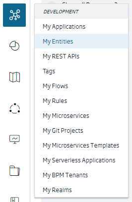
First of all, you are going to create a Platform Entity of type Entity in Historical Database, where you will store the information. To do this, navigate to the Development > My Entities menu.

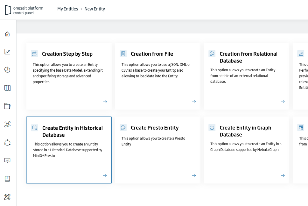
From the list of entities, press the «+» button located in the upper right part of the screen to launch the entity creation manager.

Among the different options, choose «Create Entity in Historical Database»:

This will open the Entity creation wizard, where you will have to fill in the following information:

Identification: the unique identifier of our Entity. For the example: «diabetes_raw».
Meta-Information: set of terms that define the entity. For the example: «Diabetes, Dataset, ML».
Description: a short descriptive text of the entity.

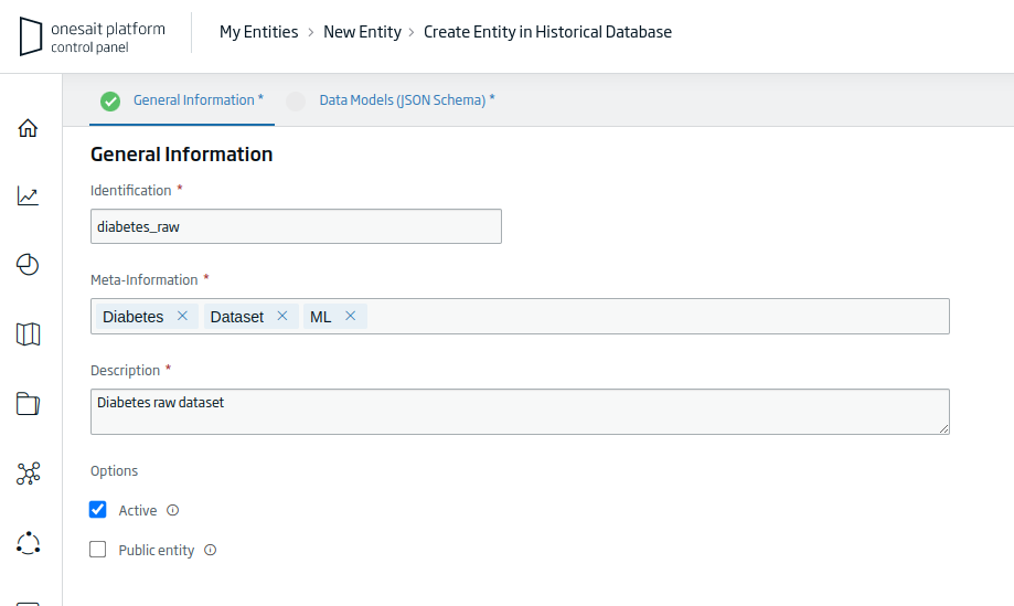
Once you have filled out the information requested, click on the «Continue» button to continue with the creation process.

Next you will have to fill all the file’s columns with the string format; it has to be done like this because the CSV file needs to be loaded with this type of column.

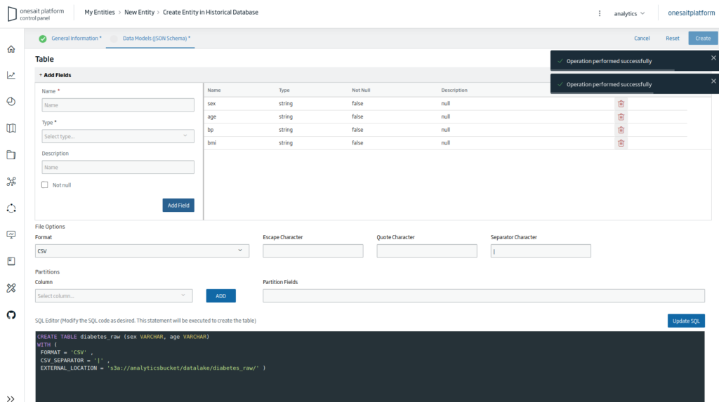
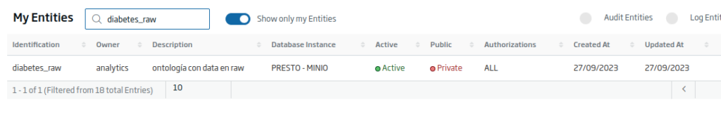
Finally, press the «Create» button to finish creating the Entity. Once done, you will return to the list of entities, where, if you search, you will see the Entity that you just created.

Step 2: Obtain data, train and record the experiment

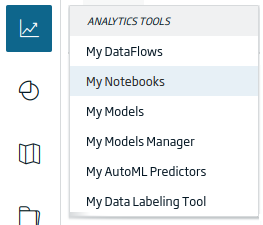
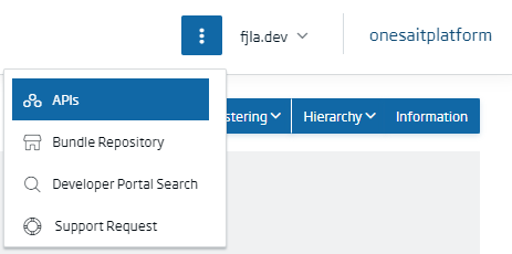
Next you are going to create a Notebook. To do this, navigate to the Analytics Tools > My Notebooks menu.

You can also import the following file, which contains the complete Notebook for this example (you would only have to set the «token» parameter).

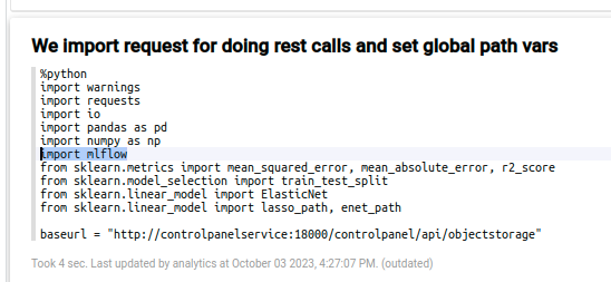
Although there are some descriptive paragraphs for the data set, you will have to go to the code section; the first paragraph corresponds to the import paragraph.

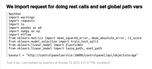
In that paragraph, the necessary libraries are loaded, and the base URL for the MinIO repository is established.

In the following paragraph, the parameters parameters are defined in order to establish variables that can come from outside.

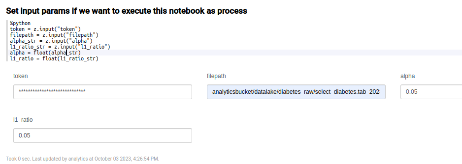
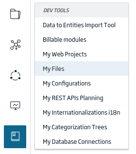
You can obtain the full path of the file, directly from the file uploaded to the Platform. To get to it, navigate to the Dev Tools > My Files menu.

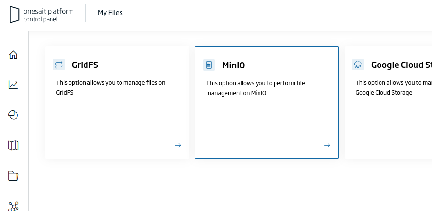
In the file selector, choose «MinIO»:

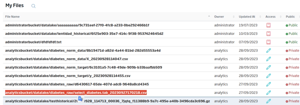
In the list of files that will appear, you can obtain the file path.

Regarding the token to use, you will use some X-OP-APIKey token that can access the file, and which is obtained from the Control Panel API manager.

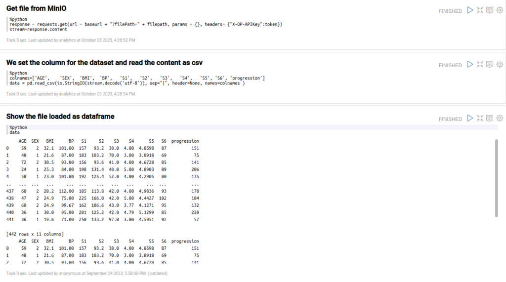
Next, in three sections, you will load the CSV file itself and the filepath from the previous section, which you will read as CSV with the dataset column (you will need to include the columns in the read_csv function) and display the loaded content.

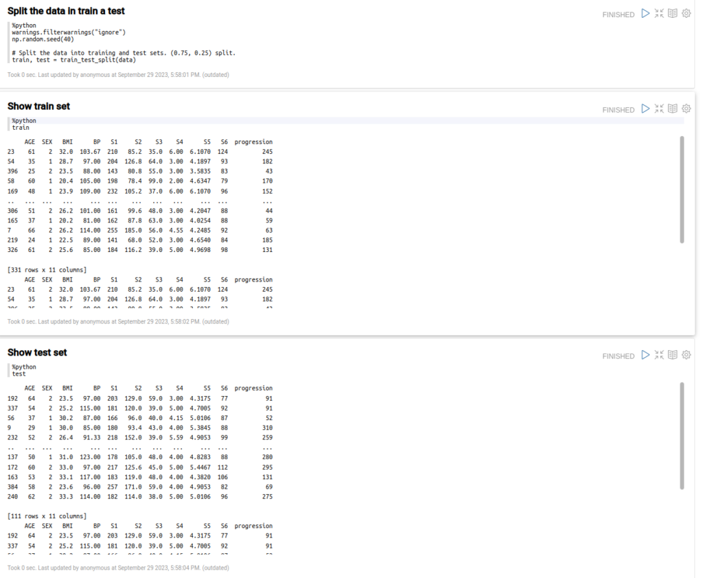
Now that you have the file as a Pandas dataframe, you can split the data into training and test sets.

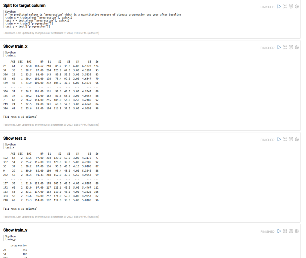
Divide these data sets also into X and Y data sets for the input parameters and expected results.

Next, with this data, execute the ElasticNet training and obtain the output model in «lr».

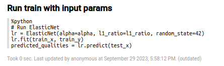
Finally, evaluate some metric for the prediction result.

Step 3: Register training and model data to MLFlow

The Notebook Engine is integrated with the MLFlow tracking service, so the only thing you have to do in the Notebook is import the necessary «MLFlow» library and use the MLFlow tracking functions.

You can do this in the import libraries section.

The connection parameters and environment variables are already done, so now you can register the parameters in MLFlow directly like this:

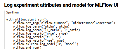
This is the standard code for tracking an experiment in MLFlow. Include everything inside «with mlflow.start_run()» to start a new experiment.

The other functions are:

mlflow.set_tag(“mlflow.runName”, …): optional property, to set a run name for the experiment. If not used, you will only have an auto-generated id, which will be the ID of the experiment.
mlflow.log_param(…): logs an input parameter for the experiment.
mlflow.log_metric(…): logs an output parameter for the experiment.
mlflow.sklearn.log_model(lr, “model”): logs and saves the trained model with all necessary metadata files.

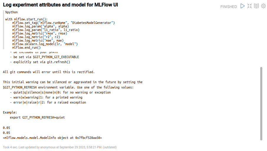
If you execute this paragraph, you will have an output similar to the following (the registration process has finished successfully):

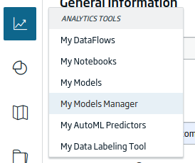
Now, move to the Models manager user interface, which you find in the Analytics Tools > My Models Manager menu.

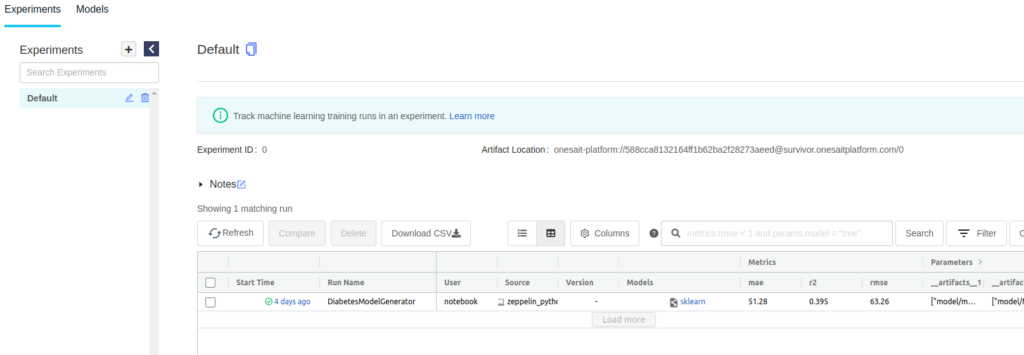
From here, you can see the execution of the experiment with all the recording parameters, metrics and files.

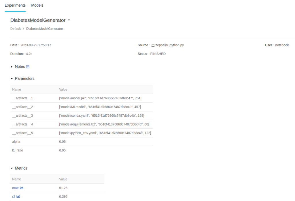
By clicking on the experiment, the details page will open:

At the end of the page, you will be able to review all the files of this experiment and the model itself:

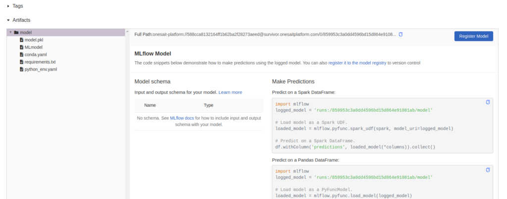
The run id on the right, named «runs:/859953c3a0dd4596bd15d864e91081ab/model», is important because you are going to use it to publish the model in the next step. This is the reference you need to collect the model in MLFlow and do some evaluations with it.

You can also register it in order to tag it, version it and have it outside the experiment. You can either do it with code, or you can use the «Register» button on the right side:

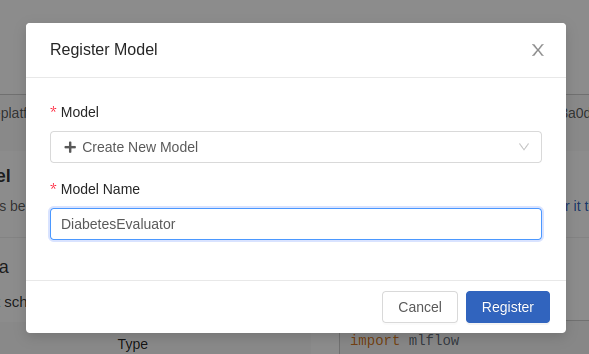
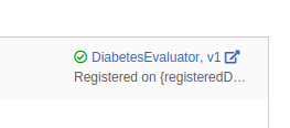
Once registered, a notification will appear on the screen.

Step 4: Create a Serverless function in Python that evaluates the data against the MLFlow model

With the model generated above, you are going to create a Python function that, with a single or multiple input, is capable of obtaining a prediction using the model.

The first step is to go to the Development > Serverless Applications menu.

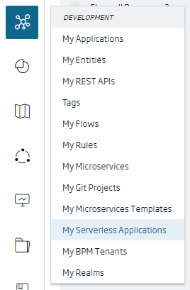
After opening the list of available applications, create a new one by clicking on the «+» button located in the upper right.

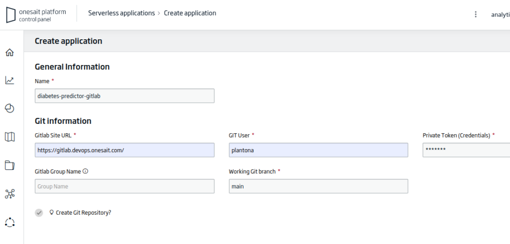
After opening the application creation wizard, you will have to fill in the following information:

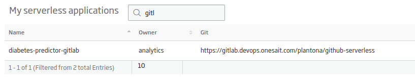
Name: the name of your application. For the example: «diabetes-predictor-gitlab».
Gitlab Site URL: the URL of the working repository. For the example: «https://gitlab.deveops.onesait.com/»
Git User: the name of the authorized user on the repository.
Working Git Branch: the branch of the repository to work on. For the example: «main».

You have the option to create a new repository or use an existing one. In any case, you will have a new application like this:

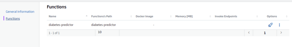
Next, you can go to the «View» button, and then to the functions tab:

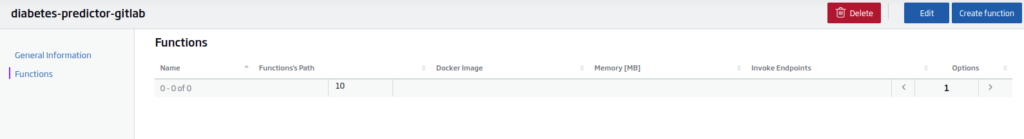
The next step will be to create or use an existing serverless function. In this case, click on «Create Function».

Once the creation wizard opens, the first step will be to select the main branch on the right side:

Next, create (either here or in the Git repository with an external editor) three files:

requirements.txt

This file will contain the libraries that your model needs to run. In this case, you will have these:

fdk
protobuf==3.20.*
numpy==1.23.4
mlflow==1.19.0
mlflow-onesaitplatform-plugin==0.2.11
scikit-learn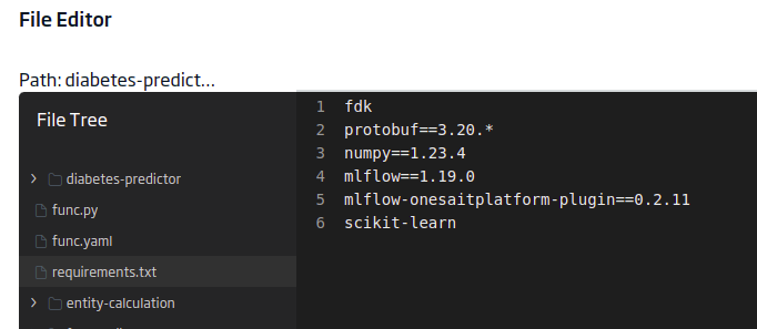

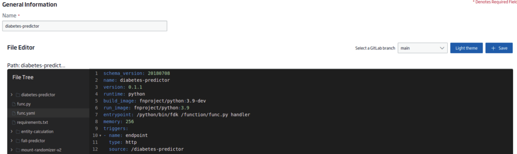
func.yaml

This other file will contain the project’s metadata required for the serverless function. The content will be:

schema_version: 20180708
name: diabetes-predictor
version: 0.1.1
runtime: python
build_image: fnproject/python:3.9-dev
run_image: fnproject/python:3.9
entrypoint: /python/bin/fdk /function/func.py handler
memory: 256
triggers:
- name: endpoint
  type: http
  source: /diabetes-predictor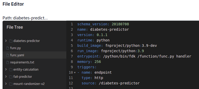

The «triggers.source» is important to have the endpoint.

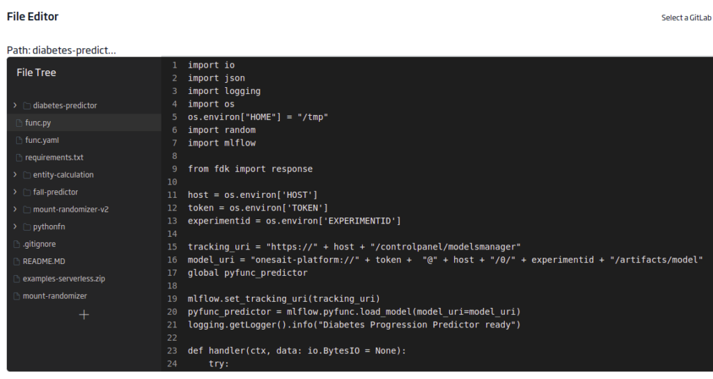
func.py

This last file contains the evaluation function itself. You will need to load the libraries to evaluate the model, MLFlow and fdk for the endpoint. An environment variable will also be used for host, experiment, and token parametric input.

import io
import json
import logging
import os
os.environ["HOME"] = "/tmp"
import random
import mlflow

from fdk import response

host = os.environ['HOST']
token = os.environ['TOKEN']
experimentid = os.environ['EXPERIMENTID']

tracking_uri = "https://" + host + "/controlpanel/modelsmanager"
model_uri = "onesait-platform://" + token +  "@" + host + "/0/" + experimentid + "/artifacts/model"
global pyfunc_predictor

mlflow.set_tracking_uri(tracking_uri)
pyfunc_predictor = mlflow.pyfunc.load_model(model_uri=model_uri)
logging.getLogger().info("Diabetes Progression Predictor ready")

def handler(ctx, data: io.BytesIO = None):
    try:
        logging.getLogger().info("Try")
        answer = []
        json_obj = json.loads(data.getvalue())
        logging.getLogger().info("json_obj")
        logging.getLogger().info(str(json_obj))
        if isinstance(json_obj, list):
            logging.getLogger().info("isinstance")
            answer = []
            values = []
            inputvector = []
            for input in json_obj:
                logging.getLogger().info("for")
                logging.getLogger().info("input: " + str(input))
                inputvector = [ input['age'], input['sex'], input['bmi'], input['bp'], input['s1'], input['s2'], input['s3'], input['s4'], input['s5'], input['s6']]
                values.append(inputvector)
                
            predict = pyfunc_predictor.predict(values)
            answer = predict.tolist()
            logging.getLogger().info("prediction")
        else:
            answer = "input object is not an array of objects:" + str(json_obj)
            logging.getLogger().error('error isinstance(json_obj, list):' + isinstance(json_obj, list))
            raise Exception(answer)
    except (Exception, ValueError) as ex:

        logging.getLogger().error('error parsing json payload: ' + str(ex))

    logging.getLogger().info("Inside Python ML function")
    return response.Response(
        ctx, response_data=json.dumps(answer),
        headers={"Content-Type": "application/json"}
    )

To save the files created as well as the changes made, as well as to deploy your function, click on the «Rocket» button of the function.

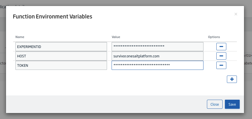
Finally, you need to add the environment variables for the model. To do this, click on the «list» button:

This will open a modal where you will fill in the information it requests:

Step 5: Model evaluation

Now, you can test the model with the REST API. You can use, for example, Postman, sending a JSON array with the input:

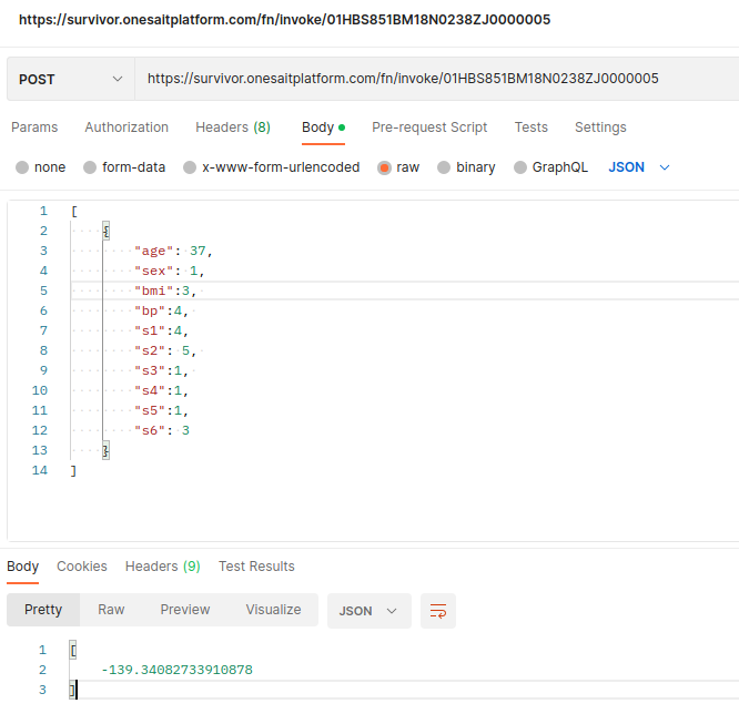
Another option you have is to create a model evaluator in the Dashboard Engine, which uses this endpoint with some input provided:

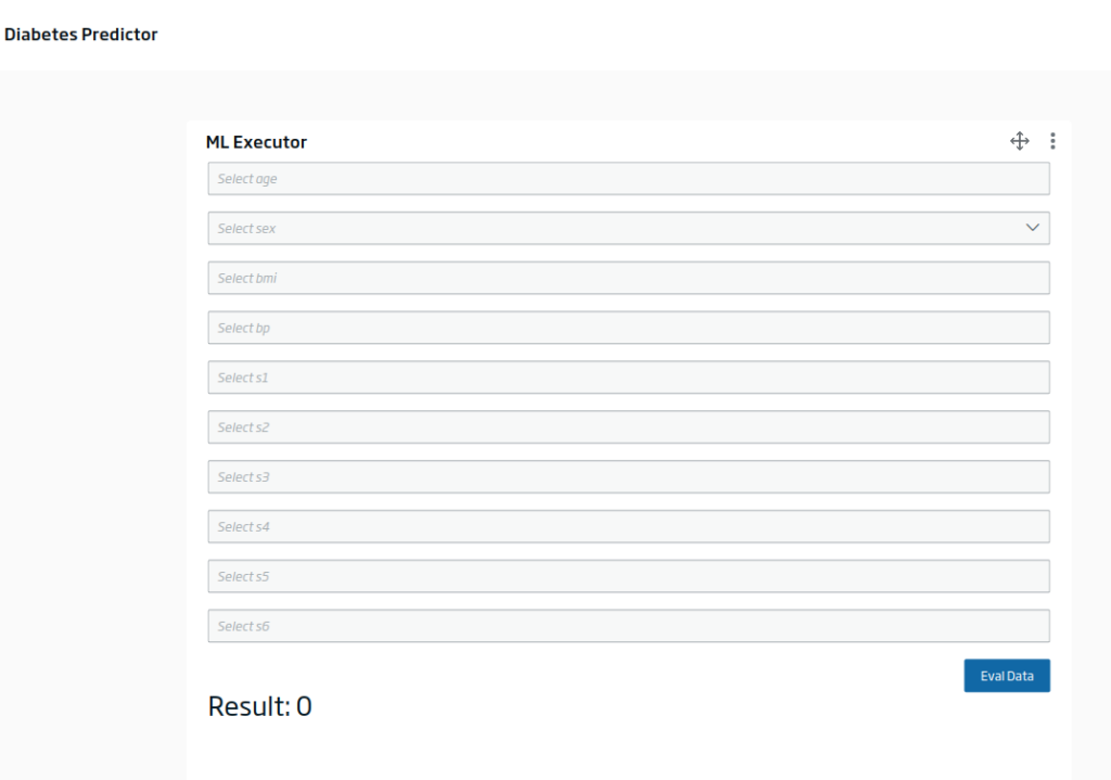
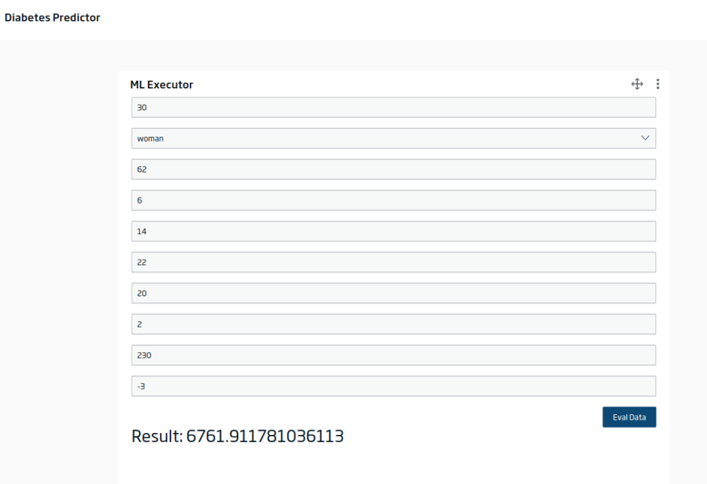
Filling in the inputs and evaluating, you would get something like this:

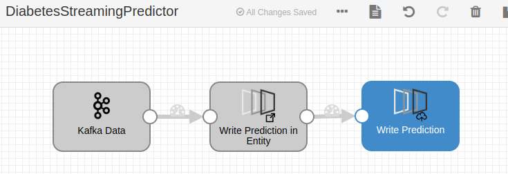
Additionally, you can evaluate the model in a batch or streaming data flow in the DataFlow with the corresponding evaluator component:

Header image: Jakob Dalbjörn at Unsplash.

Bibliografía:

Bradley Efron, Trevor Hastie, Iain Johnstone and Robert Tibshirani (2004) “Least Angle Regression,” Annals of Statistics (with discussion), 407-499 (link).