Good practices in Grafana
Grafana is the G of the EFG (Elasticsearch-Fluentd-Grafana) stack. Once an artifact sends log traces to Fluentd, which filters and transforms the data, the data are indexed in Elasticsearch. Grafana is responsible for consuming Elasticsearch traces to monitor in a very advanced graphical environment with multiple possibilities.
You can read about the basic configuration of Grafana in Kubernetes in the article on Configuration in Kubernetes that we wrote previously.
In this post, we are going to talk about some of the basic possibilities that Grafana offers. We will describe at all time real scenarios that have occurred during the work carried out in 2020Q3-4.
Study scenario
We will assume that Grafana is correctly installed and running on a server. This documentation (in Spanish) explains how to get it running on Kubernetes.
We will also assume a scenario in which structured logs in JSON format have been indexed in Elasticsearch, after passing through Fluentd. We assume that the work done so that the logs are correctly indexed and parsed in Elasticsearch is known. The articles that explain the configurations so that such a flow reaches Elasticsearch are:
Each of the fields in the JSON structure represent a key in the basic trace indexed in Elasticsearch. Let’s see it in a basic example breaking down the input and output.
Input
In this example, we assume that we have sent the following trace from a Springboot artifact via Fluentd to Elasticsearch:
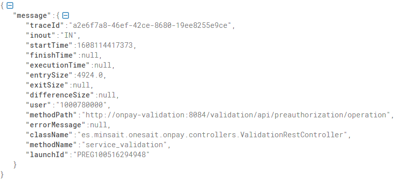
Output
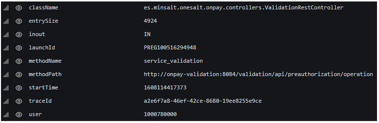
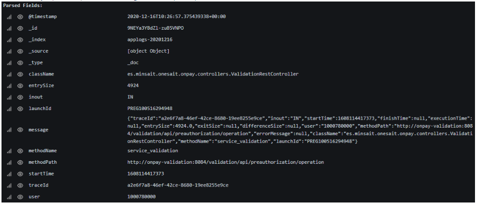
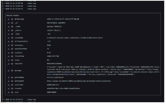
In Grafana, the example of the previous trace would be displayed as follows:
We can notice three parts:
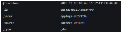
- Meta information: control and identification information indexed by Fluentd and Elasticsearch.
- Original Message: This is the JSON text that is generated in the Java artifact and persisted to the end. Bear in mind that Fluentd can cause the message in the original format not to be indexed in Elasticsearch.

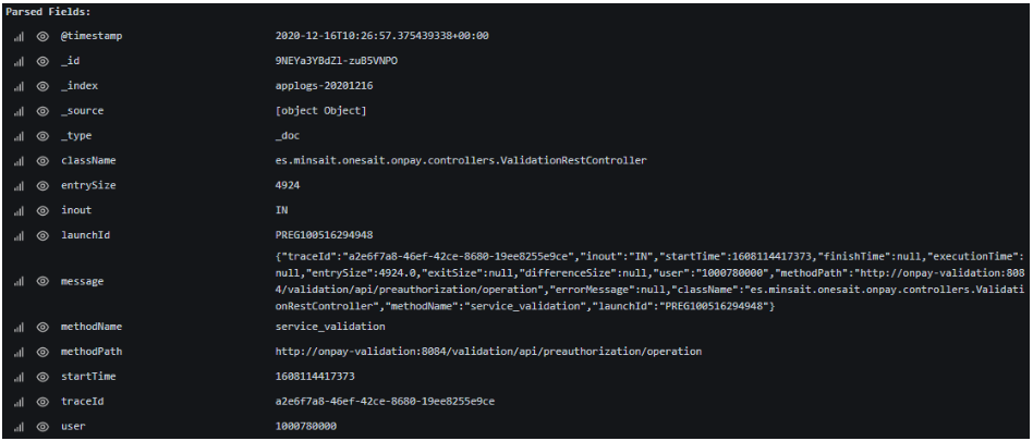
- Parsed fields: as we have said, each field of the original message is parsed and stored independently in the Elasticsearch trace. This is what will later allow us to search, display results, group, etc.
Datasource
As logical, we must tell our Grafana application where to look for the data origin. Grafana allows many Datasources, but we will focus on Elasticsearch as a basic element of our EFG stack.
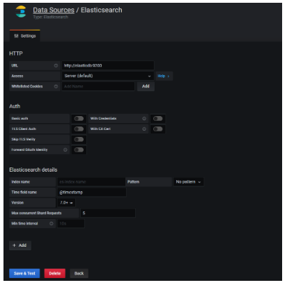
To configure the datasource, we must follow these steps:
- Configuration> Data Sources.
- Click on the «Add Datasource» button.
- Select Elasticsearch.
- Fill in the data from our Elasticsearch server. The most important are:
- HTTP: default: http://elasticsearch-host:9200
- Auth: security credentials, if applies.
- Elastic details: in this box, it is very important to correctly specify the version of Elasticsearch that Grafana is going to attack.
- Once all the basic data has been filled in, click «Save & Test».
Dashboards
A Dashboard is a set of visual panels that graphically show different sets of information. In Grafana, graphic dashboards are very versatile, and it allows them to be created and grouped in different ways, as well as adding various graphics to them.
As an extension of the «Explore» section, which we will see later, this is one of the most powerful features of the tool, since it allows you to create fixed configurations of graphs that provide the desired information at a glance, as well as the possibility of creating «playlists» (panels that rotate automatically) or «snapshots».
The visual management of the dashboards is intuitive enough not to need an additional explanation. As we said, this versatility is one of its strengths, but the real power lies in the underlying engine, the query generator, which is where the data displayed on the dashboards comes from. This is what we are going to look at, extensively, in the next section.
Export
Dashboards are especially useful when we want to export data to Excel, CSV, etc.
To do that, we must follow these steps:
- Click on the title of the panel that represents the data to be exported.
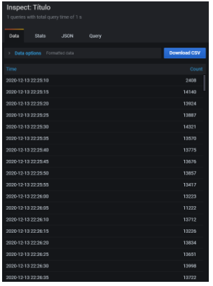
- Select Inspect > Data.
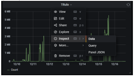
- In the panel that appears on the right, select the format in which we want to export and click «Download CSV».
Explore
As we said, the power of Grafana lies in the query generator, which can be found in the Explore section. Bear in mind that the same thing that we find in Explore, will also be found in the dashboards part, but we can consider Explore as a «training ground» with which we can generate queries that we will then take to the dashboard to assemble the desired visual representations.
By default, the Explore tool is loaded with a general search that displays results in Histogram and Table formats for samples from the last hour.
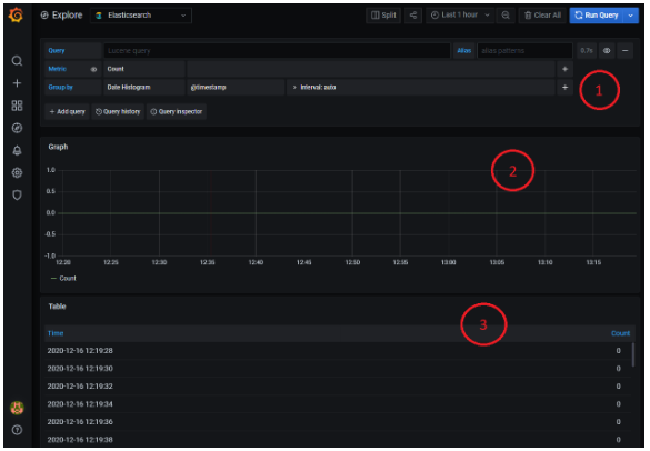
We will now analyze the different parts of the image:
- In the upper right corner there is the time range for which the search is configured. It can be selected through the selector itself at the top of the screen, or by selecting a range in the histogram with the mouse.

- To the left of the time range selector, there is a button that allows you to split the screen in two, which is useful to compare two queries.

- The area labeled with a «1» represents the query generator itself. We will go into more detail about it a little later..
- The area labeled with a «2*» is the histogram graphical representation of the requested sample. In this initial case, it is a simple count of traces per time unit.
- The area labeled with a «3*» is the tabular representation of the same result. Each row represents, in this case the traces, every 20 hundredths.
- The result panels (2 and 3) change their format and layout depending on what information is requested in the query generator. Log traces are not represented in the same way as a time panel or a histogram. We’ll look at it a bit more in detail when we talk about the query generator.
* Bear in mind that the image represents a search that has not returned any results.
Query generator
The query generator is at the top of the screen. In it, the searches themselves are configured. It is composed of:
- Query: allows you to enter queries on the fields indexed in Elasticsearch. The syntax is as described by the Apache Lucene project (Query Parser Syntax).
Let’s go back to the example where we had the following fields mapped:
A possible query to enter in the Query field, which would obtain the trace of the image, among possibly many others, is:
launchId:PREG100516294948 AND startTime:[1608114410000 TO 1681608114420000]
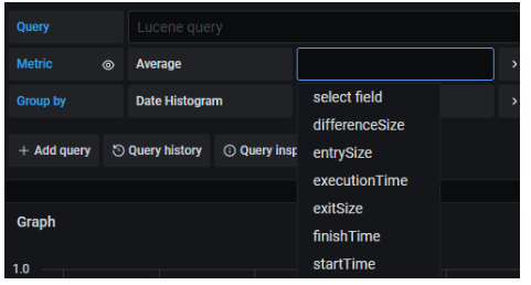
- Metric: in this field we select the metric that we want to represent, to apply to the data obtained from the query. The different values are those of the following image. Next, we detail the most used ones:
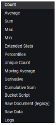
Those that apply to numerical fields require the additional selection of the field on which the metric is to be applied. For example, if Average is selected, a field will be enabled to the right of it in which we can choose between the different numerical fields found in the indexed trace.
An exception is the Count value (the first in the list), which does not require selecting the additional field, since it is about counting the number of traces found per unit of time according to the query specified in Query.
Another of the relevant values that can be chosen in the Metric field is «Logs». This is the value that must be selected if we want to enter the complete content of the traces. To clarify, there is a recurring image that we frequently go to in this article. Well, this image is the detail of a complete trace, and it is obtained by putting the aforementioned «Logs» value in the Metric field. As seen in the image below, a structured list of all* the traces that meet a certain query is obtained and, when clicking on one of them, its details are displayed:
* Bear in mind that this visualization in «Logs» format has an established limit. To see any trace, it must be found by correctly narrowing the search in the Query field.
- Group by: most of the metrics that can be selected as explained in the previous point, by default have an output in the form of a histogram (points per unit of time):
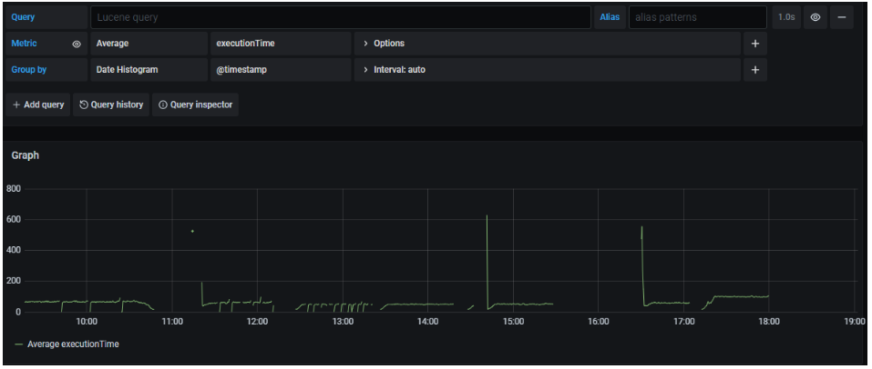
The Group by field allows grouping those obtained values based on a grouping criterion.
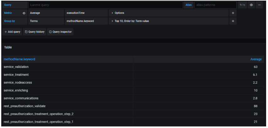
In the previous image we can see how the values obtained for the average of the executionTime field are no longer shown in a histogram, but instead a table is shown. Each row represents a different value of the field selected to group (methodName.keyword), establishing for each of them what the average executionTime is.
Both executionTime and methodName are two keys that exist in every trace indexed in Elasticsearch.
The query generator has many more possible configurations, such as the display of the query history, the inspector, and many options depending on the metrics and groupings chosen. It also allows you to create several queries (+ Add query), which would successively display several result panels (one for each configured query).
Header image: Grafana.